The theory of costs underpins the theory of supply covered in Unit 2.2. There are two ways of looking at costs, implicit costs and explicit costs.

Implicit costs

An implicit cost is the opportunity cost that exists in every business decision-making situation.

This is called an implicit cost of production because it is not stated in money terms but arises whenever a business chooses between alternatives.

Explicit costs

Explicit costs are business costs that firms incur in their operations. 

Explicit costs can be expressed in terms of the cost of factors of production:

• Land cost is rent
• Labour cost is wages
• Capital cost is interest
• Enterprise/entrepreneur cost is normal profits

The short-run (production stage)

The short-run is the time period where at least one factor of production is fixed (normally capital) while other factors such as labour can be varied.

Firms operate in the short run which is why it is called the production stage.

The long-run (planning stage)

The long-run is the time period where all factors of production are variable. 

The theory of product

The theory of product is the quantitative way the output of a firm can be expressed in the short run.

There are three ways of measuring a firm’s product:

• Total product (TP): is the total output a firm can produce from a given quantity of labour and capital inputs
• Marginal product (MP): is the change in TP when one extra unit of labour is added (ΔTP/Δ labour input).
• Average product (AP): is the output per unit of labour input (TP/ labour input)

---

The table below sets out the product data for a firm producing tables

Labour employed	total product (TP)	marginal product(MP)	Average product(AP)
1	4	4	4
2	12	8	6
3	21	9	7
4	28	7	7
5	30	2	6

 

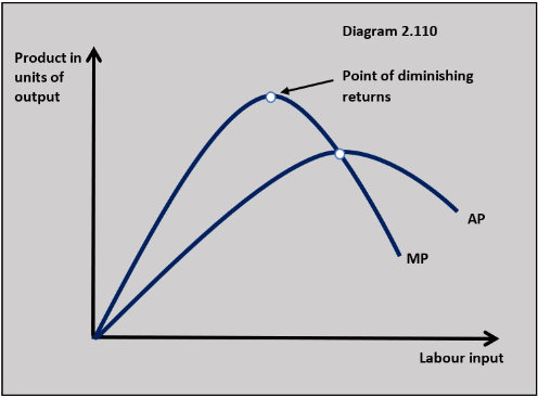
The law of diminishing returns

The law of diminishing return states that when a variable factor, such as labour, is added to a given set of fixed factors, such as capital, there is a point where the marginal product of the extra unit of variable factor added falls (diminishes).

In this table manufacturing example, the point of diminishing returns sets in when the fourth worker is added, marginal product is lower than is the case with 3 workers.

Diagram 2.110 sets out marginal and average product when more unit of labour is employed and how marginal and average product are affected by the law of diminishing returns.

---

Classifying short-run costs

Total cost (TC) is the value of all costs of producing a good.

Average total cost (ATC) is the total cost of producing each unit of a good (TC / Q = ATC).

Marginal cost (MC) is the cost of producing an extra unit of a good (change in TC / change in output = MC).

The effect of the law of diminishing returns on MC and ATC

The table below shows the cost and output data for the table manufacturer. The data shows that as output increases MC and ATC both decrease and then increase which shows the effect of the law of diminishing returns on MC and ATC.

Table 2

Output of tables	Total cost	Marginal cost	Average total cost
4	120	30.00	30.00
12	160	5.00	13.33
21	200	4.44	9.52
28	240	5.71	8.57
30	280	20.00	9.33

 

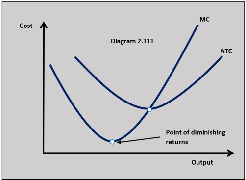Diagram 2.111 shows the link between the law of diminishing returns and MC and ATC.

When a firm starts producing the MP and AP increase at first which means that MC and ATC fall initially, but once the law of diminishing returns sets in MP and AP fall which makes MC and ATC rise. 

---

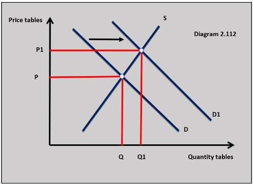The supply curve in a market is determined by the marginal cost curves of all the firms in the market. This is called horizontal summing.

This means the upward slowing nature of the market supply curve is determined by the law of diminishing returns.

---

Questions

The data in the table is production and cost data based on the production of coffee tables by a furniture manufacturer.

*Total product is the total number of high-quality coffee tables that can be produced in 12 hours with a fixed amount of capital and with different quantities of labour.

a. Outline the difference between fixed and variable costs. [2]

Fixed costs do not change with a firm’s output. Variable costs do change with a firm’s output.

b. (i) Using the data in the table, calculate the marginal product for the different quantities of labour employed. [2]

---

(ii) Using the data in the table, outline the relationship between marginal product and the quantity of labour employed. [2]

As the quantity of labour employed increases marginal product increases to the point when two workers are employed, but as the third worker is added marginal product falls and this continues when the fourth and fifth workers are added.

b. (i) Define the term the law of diminishing returns. [2] 

The law of diminishing return states that when a variable factor such as labour is added to a given set of fixed factors such as capital there is a point where the marginal product of the extra unit of variable factor added falls (diminishes).

 (ii) Using the marginal product data in the table, identify the point where diminishing returns set in. [1]

When the third worker is employed.

c. (i) Using the data in the table, determine the marginal cost and average cost figures for the different quantities of total product and complete the average and marginal cost columns in the table. [4]                                     

---

---

(ii) Draw a cost curve diagram that represents the relationship shown by the marginal cost and average total cost data in the table.  [2]     

---

• 
• 
•