Definition of PES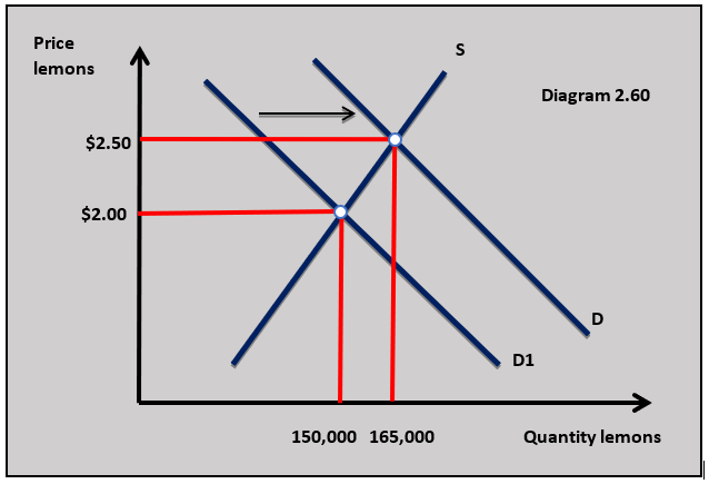

Price elasticity of supply is the responsiveness of the quantity supplied of a good to a change in its price.

PES is measured by the equation:

 % change in Qs / % change P = PES

Example of PES

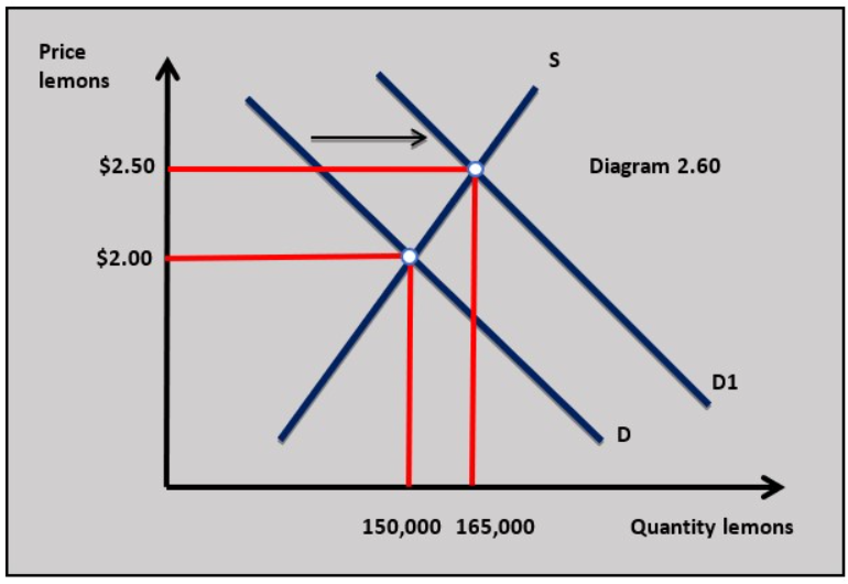
For example, if the price of lemons increases from $2 per kg to $2.50 per kg (25%) and quantity supplied increases from 150,000 kgs to 165,000 kgs (10%): +10% QS / +25% P = +0.4

This is shown in diagram 2.60. 

---

The value of PES is normally positive because of the law of supply.

In the lemon example, the PES value of +0.4 means that for every 1% increase in the price of lemons, the quantity supplied increases by 0.4%.

Price elastic supply

If the PES value is greater than 1 then the good’s supply is price elastic.  This means a change in price leads to a proportionately greater change in quantity supplied.

For example, a 5% increase in the price of copper leads to a 10% increase in the supply of copper, the PES would be: +10% QS / +5% P = +2.0 PES 

Theoretically, the supply curve can be perfectly horizontal or perfectly elastic. This gives a PES of infinity. 

Unitary elasticity of supply 

If the value is 1 then PES is unitary. 

This means that for every 1% change in price, the quantity supplied changes by 1%.

Any straight-line supply curve that passes through the origin has a PES value of 1.

Price inelastic supply

If the supply of a good has a PES of less than 1 then its supply is price inelastic. 

This means that a change in the price of a good leads to a less than proportionate change in quantity supplied. 

For example, if the price of oat milk rises from $2 per unit to $2.80 and quantity supplied increases from 10,000 units to 12,000 units supplied the PED is calculated as: +20% QS / +40% P = 0.5 PES

Theoretically, the supply curve can be perfectly vertical or perfectly inelastic. This gives a PES of 0.

Diagram showing different PES

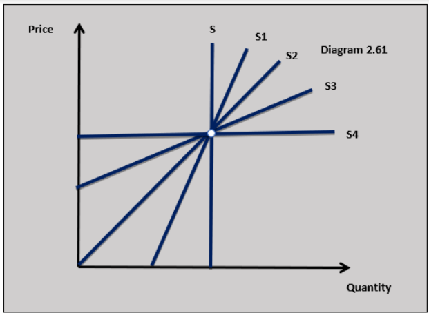
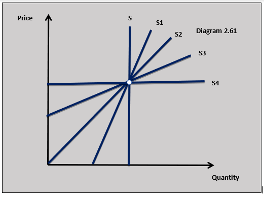Diagram 2.61 shows supply curves of different elasticities. 

• Vertical curve is perfectly elastic (S)
• Relatively steep gradient is price inelastic (S1)
• Straightline through the origin unitary elasticity (S2)
• Relatively flat gradient is price elastic (S3)
• Vertical supply curve is perfectly inelastic (S4)

---

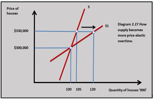
Time

In the short run, the supply of a good tends to be inelastic because producers find it difficult to increase output when the factors of production used to produce the good are difficult to change quickly.

In the long-run, the supply of a good becomes more elastic because producers find it easier to respond to an increase in price.

Availability of factors of production

The easier it is for producers to access factors of production, the more elastic PES tends to be. 

Supply tends to be more elastic when businesses are generally quick to set up and operate because the land, labour and capital needed are relatively accessible.

When resources are relatively difficult to access supply tends to be more inelastic because costs tend to rise quickly when producers try to increase output.

Stock and used capacity

Where producers have spare capacity and available stock, supply tends to be relatively price elastic because producers can more easily meet demand when price increases. 

 

Commodities

The supply of primary commodities tends to be relatively inelastic because it is difficult for producers to respond to a change in price. 

The supply of the agricultural sector, for example, is limited by the growing seasons of farmers. 

---

Manufactured goods

The supply of manufactured goods is more price elastic in comparison to primary products because producers can change supply in response to a change in price more quickly. 

Manufacturers are not limited by environmental factors such as growing seasons. 

Manufactured goods can also be stored more easily than agricultural goods which tend to be perishable. 

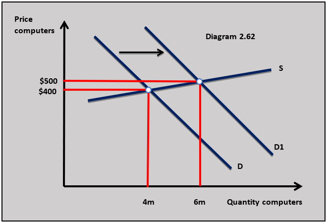
Diagram 2.62 shows price elastic supply for computers as a manufactured good. The example here is a 25% increase in price leads to a 50% increase in quantity supplied.

The PES would be: +50% QS / +25% P = +2.0 PES 

Explain two reasons why the supply of certain manufactured goods might be relatively price elastic. [10]

Definitions of price elasticity of supply, manufactured goods and price elastic supply.

A diagram to show price elastic supply of a manufactured good such as cars.

An explanation that the supply of a manufactured good such as cars is price elastic because it is possible to hold stocks of cars and release stock onto the market to increase quantity supplied if prices rise.

---

An explanation that if manufacturing businesses have the spare capacity it is possible to increase quantity supplied relatively easily if price increases.

---

• 
• 
• 
•